Spring 2022:
ERS Post-Launch Data Challenge #1: Simulated Data

The Transiting Exoplanet Community ERS team conducted a data challenge exercise based on simulated data during the JWST commissioning period. The event was held March 21-23, 2022 in-person at Baltimore, MD, USA and Heidelberg, Germany, with opportunities for remote online participation. This was an opportunity to try lots of different analyses and learn together as a community how to work with the new challenges of JWST data.

(The description below was last updated March 20, 2022.)

Goals

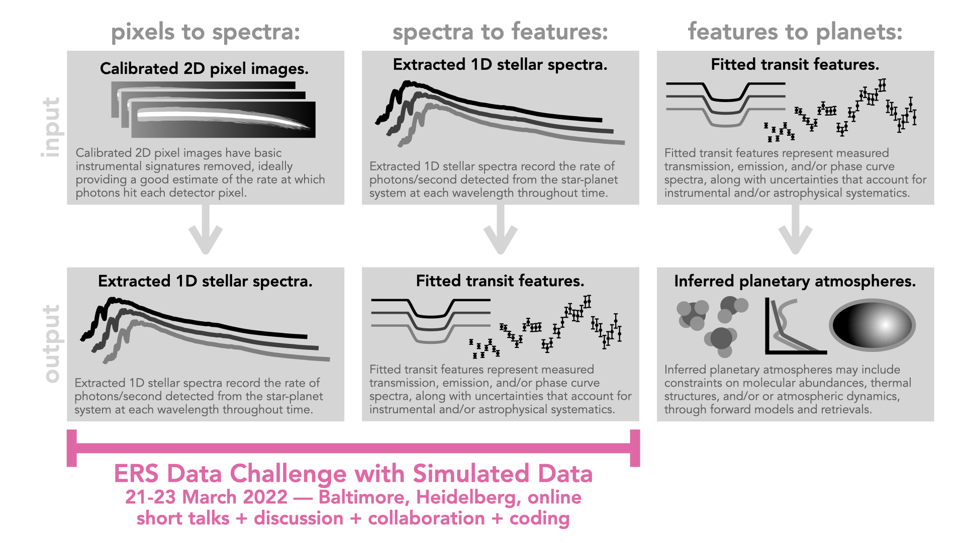
1. Develop and exercise open-source tools for JWST data analysis to go from detector pixels to time-series stellar spectra
2. Develop and exercise open-source tools for JWST data analysis to go from time-series stellar spectra to fitted planetary features
3. Perform meaningful intercomparisons of analysis tools, including those developed by STScI
4. Compute planetary spectra and meta-data from simulated data, and make them available to community for retrieval studies
5. Generate draft analysis cookbooks with simulated data, as a practice run for incoming real data and the autumn program deliverables

Agenda + Local Logistics

The agenda for the March 21-23, 2022 meeting is available here, covering participants in Baltimore, Heidelberg, and online. Most of the time is budgeted for open work, so you can get whatever you want out of the week!

Local logistics information for in-person Baltimore attendees has been emailed to all registered Baltimore participants, and a summary is available here. Local logistics information for in-person Heidelberg attendees has been emailed to all registered Heidelberg participants. Connection information for remote participants has been shared over slack and email to all registrants.

The ers-transit Data Simulation Working Group has produced a suite of data simulations for the Spring 2022 data challenge, designed to approximate the real datasets that will actually be gathered by JWST. These simulated datasets include injected planetary signals, they include outputs at multiple different processing steps, and they provide a good overall sense of the data products that expected for each instrument. Although the real observations will certainly contain unexpected features or aspects that are difficult to model from scratch, these simulations should serve as a useful starting place to develop, test, and compare your analysis methods.

Types of Data Products

For each simulated observation, data products are provided at various stages of processing. In general, the size of datasets decreases from least processed (raw ramp data) to most processed (spectra or light curves).

• uncalibrated raw data (Stage 0) = These are time-series sets of pixel images for individual readout groups, showing some or all of the non-destructive detector reads that make up each integration. (To learn about JWST’s language of frames, groups, integrations, and exposures, see Understanding Exposure Times.) Minimal processing has been applied to these raw images. Files look like `*uncal.fits` and are multi-extension FITS images.
• countrate images (Stage 1) = These are time-series sets of pixel images for individual integrations, showing the rates at which photons hit the detector. These images are corrected for bias levels, dark current, and non-linearity, they have been checked for saturation, the reference pixel correction has been applied, and a slope has been fit to the individual groups within an integration (the “ramps-to-slopes” process). Files look like `*rateints.fits` and are multi-extension FITS images.
• calibrated flux images (Stage 2) = These are time-series sets of pixel images for individual integrations, with various additional calibrations applied. Visually, they will likely look very similar to countrate images, but pixels have been converted from photons/second to astrophysically calibrated flux units (MJy), each integration now has a wavelength solution assigned, and some trimming may have been applied. Files look like `*calints.fits` and are multi-extension FITS images.
• time-series extracted 1D spectra (Stage 2 or 3) = These are time-series sets of extracted stellar spectra for individual integrations. These represent the flux of the star-planet system as a function of wavelength and time. Integrated across any particular wavelength range, they would provide a light curve. Integrated across any particular time range, they would provide an average stellar spectrum. Files look like `*x1dints.fits`and are FITS binary tables.
• integrated broadband light curves (Stage 3) = These are text files containing columns for time and broadband, integrated, flux over the entire spectrum for each individual integration. These are the literal sums along the wavelength-axis of the 1D spectra contained in the `*x1dints.fits` files (described above). These files exist for both the spectroscopic and photometric (NIRCam only) data. Files look like `*.ecsv` and are Enhanced Character Separate Values text files.

The `jwst` documentation Science Products and Data Product Types pages explain the formats of these files and what processing steps have likely gone into them. Néstor Espinoza’s talk from the ERS Pre-Launch Data Hackathon (slides, video) provides a comprehensive pedagogical introduction to JWST datasets and the language used to describe them, with particular relevance to time-series observations and exoplanet datasets.

All public datasets created by the Data Simulation Working Group are available through this Box folder, including both those for the upcoming Spring 2022 Data Challenge and those from the previous Summer 2021 Pre-Launch Data Hackathon. The list below links directly to folders of simulated data for each of four simulated observations. Details about the inputs, assumptions, and processing are provided in README files associated with each simulated dataset. No login is required.

• NIRISS | WASP-39b Transit
  • A single transit
  • SOSS spectroscopy spanning 0.6-2.5 microns (SUBSTRIP256) at R~700
  • Available data products: Stage 0, 1, 2
• NIRSpec | WASP-39b Transit
  • A single transit
  • PRISM spectroscopy spanning 0.6-5.0 microns (SUB512) at R~100
  • Simulations were generated by injecting a transit signal into real cryo-vacuum test data from ground testing of the instrument
  • Available data products: Stage 1, 2
• NIRCam | WASP-39b Transit
  • A single transit.
  • F322W2 spectroscopy spanning 2.4-4.0 microns at R~1700, with simultaneous F210M filter photometry at 2.1 microns
  • Simulations were generated with and without additional systematics.
  • Available data products: Stage 0, 1, 2, 3
• MIRI | NGTS-10b Phase Curve
  • A full planetary orbit, including one transit and two eclipses.
  • LRS spectroscopy spanning 5-12 microns at R~100.
  • Simulations were generated with and without detector pixel response drift.
  • Includes a nearby non-target star in the field of view.
  • Available data products: Stage 0, 1, 2.

This first post-launch ERS data challenge meeting is meant to serve as an opportunity for as many people as possible to start analyzing simulated data and preparing for the real JWST datasets that will be coming soon. We hope to engage as many scientists as possible in attempting independent analyses of the simulated datasets, to learn as much as we can as a community of JWST observers, and to discover areas where we future. The March 21-23 event will focus primarily on the steps between detector pixels and fitted planetary features, but we welcome contributions focused on other tools, models, or observations relevant to the ERS program.

Contribute a Draft Analysis:

Everyone can participate in the “pixels-to-features” data challenge activities leading up to the March 21-23 meeting. We encourage you to try something, even if it’s not perfect. The more folks we have working on the simulated data, the more we’ll learn and the better prepared we will be for the real data when it arrives! Here’s what to do:

1. Register for the Spring 2022 Data Challenge with Simulated Data. Even if you are not planning to synchronously attend the meeting, we will use the contact list from this form to communicate with everyone working on the datasets. (Late registrations are OK, except for in-person participants!)
2. Choose one or more simulated dataset(s). Pick a simulated observation you are excited to work on, either because you want to contribute to the analysis of that observation for the ERS program or because you have another similar observation of your own and you want to become familiar with the data.
3. Choose one or more analysis step(s) that you want to attempt for that simulated observation. Below, we describe a few Data Product Checkpoints in the process from detector pixels to fitted features. You can start and finish wherever you like, but if you work on more than one step, please consider submitting intermediate data products to line up with the checkpoints described below.
4. Join the #dc-general channel on the ers-transit slack to learn about updates and be able to discuss on-going issues with other members of the ers-team. Weekly online “studio sessions” will be organized for folks who want to work companionably on their data analysis efforts. If you're not on the ers-transit slack workspace, please contact us.
5. Submit your results by 14 March 2022. Please submit the data products associated with your analysis step(s), along with any visualizations or descriptions of your results that will be helpful for others to follow your work. The Data Product Checkpoints defined below are the places at which your submitted results can be visualized, evaluated, and compared to injected signals.

Our goal for this event is not to have all the perfect answers for the optimal method to analyze JWST data. Our goals are to explore and discover what we can. If the data products you submit are not perfect, that’s OK! We plan to include lots of time during the March 21-23 meeting for folks to discuss, learn, and work together to try to improve all our analyses!

The Data Challenge Working Group is assembling a suite of tests that can be applied at various checkpoints in the data analysis process. You can submit results at any of these checkpoints, and then the DCWG will generate visualizations and calculate data quality metrics for your submission. These are not meant to replace your own visualizations or characterizations of your methods; they are meant simply to provide an easy way to compare results to injected signals (wherever possible) and to look at multiple analyses in a uniform way. The following list summarizes the types of data analysis checkpoints that we hope to investigate. It will ease comparison if you match the requested file formats as closely as possible and include a short README with any submissions.

• countrate images = If starting from raw uncalibrated data, what per-integration countrate images are produced? What are the detector noise levels, what fractions of pixels identified as bad or cosmic rays, and what spatially or temporally correlated background trends are present? You can submit: a collection of countrate images. These should be equivalent to `*rateints` files, containing values and uncertainties in units of DN/second. (One particular data segment file will be suggested as a testbed for this checkpoint.)
• background-subtracted countrate images = One area of particular concern for extracting spectra is understanding how to most accurately subtract image backgrounds caused by astrophysical flux and/or detector noise patterns. You can submit: a collection of countrate images with the backgrounds subtracted from them. These should be equivalent to `*rateints` files, containing values and uncertainties in units of DN/second. (One particular data segment file will be suggested as a testbed for this checkpoint.)
• time-series extracted 1D spectra = If starting from countrate images and/or calibrated flux images, what time-series stellar spectra are produced? What is the precision of the extracted flux across time and wavelength, how accurate are the fluxes, what correlations across time or wavelength are present in the noise, and how common are outliers? You can submit: a collection of time-series extracted spectra, including flux values and uncertainties for each wavelength and time (= integration) in the original dataset. Your data may optionally include additional metadata or time-series diagnostics. Any flux units are allowed (including normalized to unity), as long as they are consistent between the flux and its uncertainty. The chromatic package will be used to load your submissions; please submit in a file format for which a file-reader already exists or work with the DCWG to implement a new reader for your specific format.

The time-series extracted 1D spectra for JWST instruments have hundreds to thousands of wavelengths. For some datasets, it may be useful to fit transit features at high spectral resolution, but for this event we suggest that you bin the data onto a coarser grid of wavelength bins to simplify fitting and comparison. If you want to be able to compare directly to others' results, use the following effective wavelength bins. This notebook provides more details on the suggested bins, including copy-and-paste values for the bin indices and wavelength values.

• binned light curves and residuals = After binning spectra into wavelength bins, what do the light curves look like and how well can they be modeled? What is the noise like, how many outliers are there, what systematics are present, and how well can models capture all aspects of the data? You can submit: a collection of wavelength-binned light curves to which some model has been fit. These should be a text file (or collection of text files) containing time, per-wavelength fluxes, per-wavelength flux uncertainties, and per-wavelength residuals from the fitted model.
• fitted planetary features = If starting from time-series spectra, what wavelength-dependent planetary features (transit depths, eclipse depths, or phase curve amplitudes/offsets) do we infer? With what precision and accuracy do fitted features match the signals that were injected? You can submit: a collection of wavelength-dependent transit depths or eclipse depths, depending on the dataset being modeled, along with their uncertainties. Transit depths should be submitted as (Rp/Rs)^2 = the square of the planet-to-star radius ratio, and eclipse depths should be submitted as (Fp/Fs) = the ratio of planet and star fluxes reaching our telescope.

Other Submissions:

You may want to contribute to this Data Challenge in a way that doesn’t neatly fall into the categories or checkpoints described above. The ERS team values creative and thoughtful contributions in areas that we did not necessarily plan. As such, there is a general opportunity to submit plots, animations, cartoons, illustrations, infographics, artwork, or any other kind of creative contribution that’s relevant to the ers-transit science program. At the March 21-23 events, we will showcase and celebrate your submissions!